半教師ありオブジェクト検出

半教師ありオブジェクト検出は、ラベル付きデータとラベルなしデータの両方を使用してトレーニングを行います。高性能なオブジェクト検出器のトレーニングにおけるアノテーションの負担を軽減するだけでなく、大量のラベルなしデータを使用することでオブジェクト検出器をさらに向上させます。

半教師ありオブジェクト検出器をトレーニングするための典型的な手順は次のとおりです。

• 半教師ありオブジェクト検出

  • データセットの準備と分割

  • マルチブランチパイプラインの設定

  • 半教師ありデータローダーの設定

  • 半教師ありモデルの設定

  • MeanTeacherHookの設定

  • TeacherStudentValLoopの設定

データセットの準備と分割

データセットのダウンロードスクリプトを提供しています。デフォルトではcoco2017データセットをダウンロードし、自動的に解凍します。

python tools/misc/download_dataset.py

解凍されたデータセットのディレクトリ構造は次のとおりです。

mmdetection
├── data
│   ├── coco
│   │   ├── annotations
│   │   │   ├── image_info_unlabeled2017.json
│   │   │   ├── instances_train2017.json
│   │   │   ├── instances_val2017.json
│   │   ├── test2017
│   │   ├── train2017
│   │   ├── unlabeled2017
│   │   ├── val2017

coco2017データセットにおける半教師ありオブジェクト検出の一般的な実験設定は2つあります。

(1) train2017を固定の割合（1％、2％、5％、10％）でラベル付きデータセットとして分割し、残りのtrain2017をラベルなしデータセットとします。train2017の異なる分割をラベル付きデータセットとして使用すると、半教師あり検出器の精度に大きな変動が生じるため、実際には5分割交差検証を使用してアルゴリズムを評価します。データセット分割スクリプトを提供しています。

python tools/misc/split_coco.py

デフォルトでは、スクリプトはtrain2017をラベル付きデータの比率1％、2％、5％、10％に従って分割し、各分割は交差検証のためにランダムに5回繰り返されます。生成される半教師ありアノテーションファイル名の形式は次のとおりです。

• ラベル付きデータセットの名前形式：instances_train2017.{fold}@{percent}.json

• ラベルなしデータセットの名前形式：instances_train2017.{fold}@{percent}-unlabeled.json

ここで、foldは交差検証に使用され、percentはラベル付きデータの比率を表します。分割されたデータセットのディレクトリ構造は次のとおりです。

mmdetection
├── data
│   ├── coco
│   │   ├── annotations
│   │   │   ├── image_info_unlabeled2017.json
│   │   │   ├── instances_train2017.json
│   │   │   ├── instances_val2017.json
│   │   ├── semi_anns
│   │   │   ├── instances_train2017.1@1.json
│   │   │   ├── instances_train2017.1@1-unlabeled.json
│   │   │   ├── instances_train2017.1@2.json
│   │   │   ├── instances_train2017.1@2-unlabeled.json
│   │   │   ├── instances_train2017.1@5.json
│   │   │   ├── instances_train2017.1@5-unlabeled.json
│   │   │   ├── instances_train2017.1@10.json
│   │   │   ├── instances_train2017.1@10-unlabeled.json
│   │   │   ├── instances_train2017.2@1.json
│   │   │   ├── instances_train2017.2@1-unlabeled.json
│   │   ├── test2017
│   │   ├── train2017
│   │   ├── unlabeled2017
│   │   ├── val2017

(2) train2017をラベル付きデータセットとして、unlabeled2017をラベルなしデータセットとして使用します。image_info_unlabeled2017.jsonにはcategories情報が含まれていないため、CocoDatasetを初期化できません。instances_train2017.jsonのcategoriesをimage_info_unlabeled2017.jsonに書き込み、instances_unlabeled2017.jsonとして保存する必要があります。関連するスクリプトは次のとおりです。

from mmengine.fileio import load, dump

anns_train = load('instances_train2017.json')
anns_unlabeled = load('image_info_unlabeled2017.json')
anns_unlabeled['categories'] = anns_train['categories']
dump(anns_unlabeled, 'instances_unlabeled2017.json')

処理されたデータセットディレクトリは次のとおりです。

mmdetection
├── data
│   ├── coco
│   │   ├── annotations
│   │   │   ├── image_info_unlabeled2017.json
│   │   │   ├── instances_train2017.json
│   │   │   ├── instances_unlabeled2017.json
│   │   │   ├── instances_val2017.json
│   │   ├── test2017
│   │   ├── train2017
│   │   ├── unlabeled2017
│   │   ├── val2017

マルチブランチパイプラインの設定

半教師あり学習には、主に一貫性正則化と擬似ラベルの2つのアプローチがあります。一貫性正則化は注意深い設計が必要となることがありますが、擬似ラベルはより単純な形式で、ダウンストリームタスクに拡張しやすいです。擬似ラベルに基づく教師-生徒の共同トレーニング半教師ありオブジェクト検出フレームワークを採用しているため、ラベル付きデータとラベルなしデータは異なるデータパイプラインを設定する必要があります。

(1) ラベル付きデータのパイプライン

# pipeline used to augment labeled data,
# which will be sent to student model for supervised training.
sup_pipeline = [
    dict(type='LoadImageFromFile', backend_args=backend_args),
    dict(type='LoadAnnotations', with_bbox=True),
    dict(type='RandomResize', scale=scale, keep_ratio=True),
    dict(type='RandomFlip', prob=0.5),
    dict(type='RandAugment', aug_space=color_space, aug_num=1),
    dict(type='FilterAnnotations', min_gt_bbox_wh=(1e-2, 1e-2)),
    dict(type='MultiBranch', sup=dict(type='PackDetInputs'))
]

(2) ラベルなしデータのパイプライン

# pipeline used to augment unlabeled data weakly,
# which will be sent to teacher model for predicting pseudo instances.
weak_pipeline = [
    dict(type='RandomResize', scale=scale, keep_ratio=True),
    dict(type='RandomFlip', prob=0.5),
    dict(
        type='PackDetInputs',
        meta_keys=('img_id', 'img_path', 'ori_shape', 'img_shape',
                   'scale_factor', 'flip', 'flip_direction',
                   'homography_matrix')),
]

# pipeline used to augment unlabeled data strongly,
# which will be sent to student model for unsupervised training.
strong_pipeline = [
    dict(type='RandomResize', scale=scale, keep_ratio=True),
    dict(type='RandomFlip', prob=0.5),
    dict(
        type='RandomOrder',
        transforms=[
            dict(type='RandAugment', aug_space=color_space, aug_num=1),
            dict(type='RandAugment', aug_space=geometric, aug_num=1),
        ]),
    dict(type='RandomErasing', n_patches=(1, 5), ratio=(0, 0.2)),
    dict(type='FilterAnnotations', min_gt_bbox_wh=(1e-2, 1e-2)),
    dict(
        type='PackDetInputs',
        meta_keys=('img_id', 'img_path', 'ori_shape', 'img_shape',
                   'scale_factor', 'flip', 'flip_direction',
                   'homography_matrix')),
]

# pipeline used to augment unlabeled data into different views
unsup_pipeline = [
    dict(type='LoadImageFromFile', backend_args=backend_args),
    dict(type='LoadEmptyAnnotations'),
    dict(
        type='MultiBranch',
        unsup_teacher=weak_pipeline,
        unsup_student=strong_pipeline,
    )
]

半教師ありデータローダーの設定

(1) 半教師ありデータセットを構築します。ConcatDatasetを使用して、ラベル付きデータセットとラベルなしデータセットを連結します。

labeled_dataset = dict(
    type=dataset_type,
    data_root=data_root,
    ann_file='annotations/instances_train2017.json',
    data_prefix=dict(img='train2017/'),
    filter_cfg=dict(filter_empty_gt=True, min_size=32),
    pipeline=sup_pipeline)

unlabeled_dataset = dict(
    type=dataset_type,
    data_root=data_root,
    ann_file='annotations/instances_unlabeled2017.json',
    data_prefix=dict(img='unlabeled2017/'),
    filter_cfg=dict(filter_empty_gt=False),
    pipeline=unsup_pipeline)

train_dataloader = dict(
    batch_size=batch_size,
    num_workers=num_workers,
    persistent_workers=True,
    sampler=dict(
        type='GroupMultiSourceSampler',
        batch_size=batch_size,
        source_ratio=[1, 4]),
    dataset=dict(
        type='ConcatDataset', datasets=[labeled_dataset, unlabeled_dataset]))

(2) マルチソースデータセットサンプラーを使用します。GroupMultiSourceSamplerを使用して、labeled_datasetとlabeled_datasetからバッチ単位でデータをサンプリングします。source_ratioは、バッチ内のラベル付きデータとラベルなしデータの比率を制御します。GroupMultiSourceSamplerは、同じバッチ内の画像のアスペクト比が類似していることも保証します。バッチ内の画像のアスペクト比を保証する必要がない場合は、MultiSourceSamplerを使用できます。GroupMultiSourceSamplerのサンプリング図は次のとおりです。

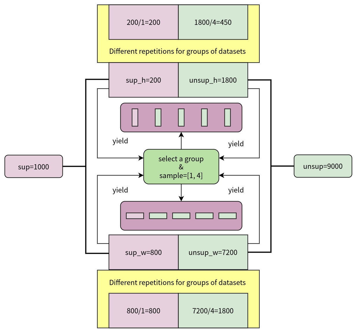
sup=1000 は、ラベル付きデータセットの規模が1000であることを示します。sup_h=200 は、ラベル付きデータセットの中でアスペクト比が1以上の画像の規模が200であることを示します。sup_w=800 は、ラベル付きデータセットの中でアスペクト比が1未満の画像の規模が800であることを示します。unsup=9000 は、ラベルなしデータセットの規模が9000であることを示します。unsup_h=1800 は、ラベルなしデータセットの中でアスペクト比が1以上の画像の規模が1800であることを示します。unsup_w=7200 は、ラベルなしデータセットの中でアスペクト比が1未満の画像の規模が7200であることを示します。GroupMultiSourceSampler は、ラベル付きデータセットとラベルなしデータセットの画像の全体的なアスペクト比分布に基づいてランダムにグループを選択し、source_ratio に従って2つのデータセットからデータをサンプリングしてバッチを形成するため、ラベル付きデータセットとラベルなしデータセットは異なる繰り返し回数になります。

半教師ありモデルの設定

半教師あり学習の detector として Faster R-CNN を選択します。半教師ありオブジェクト検出アルゴリズム SoftTeacher を例に挙げると、モデルの設定は _base_/models/faster-rcnn_r50_fpn.py を継承し、検出器のバックボーンネットワークを caffe スタイルに置き換えることができます。教師あり学習の設定とは異なり、detector としての Faster R-CNN は model ではなく、model の属性であることに注意してください。さらに、data_preprocessor は、異なるパイプラインからの画像をパディングおよび正規化するために使用される MultiBranchDataPreprocessor に設定する必要があります。最後に、半教師あり学習とテストに必要なパラメータは、semi_train_cfg と semi_test_cfg を介して設定できます。

_base_ = [
    '../_base_/models/faster-rcnn_r50_fpn.py', '../_base_/default_runtime.py',
    '../_base_/datasets/semi_coco_detection.py'
]

detector = _base_.model
detector.data_preprocessor = dict(
    type='DetDataPreprocessor',
    mean=[103.530, 116.280, 123.675],
    std=[1.0, 1.0, 1.0],
    bgr_to_rgb=False,
    pad_size_divisor=32)
detector.backbone = dict(
    type='ResNet',
    depth=50,
    num_stages=4,
    out_indices=(0, 1, 2, 3),
    frozen_stages=1,
    norm_cfg=dict(type='BN', requires_grad=False),
    norm_eval=True,
    style='caffe',
    init_cfg=dict(
        type='Pretrained',
        checkpoint='open-mmlab://detectron2/resnet50_caffe'))

model = dict(
    _delete_=True,
    type='SoftTeacher',
    detector=detector,
    data_preprocessor=dict(
        type='MultiBranchDataPreprocessor',
        data_preprocessor=detector.data_preprocessor),
    semi_train_cfg=dict(
        freeze_teacher=True,
        sup_weight=1.0,
        unsup_weight=4.0,
        pseudo_label_initial_score_thr=0.5,
        rpn_pseudo_thr=0.9,
        cls_pseudo_thr=0.9,
        reg_pseudo_thr=0.02,
        jitter_times=10,
        jitter_scale=0.06,
        min_pseudo_bbox_wh=(1e-2, 1e-2)),
    semi_test_cfg=dict(predict_on='teacher'))

さらに、RetinaNet や Cascade R-CNN などの他の検出モデルの半教師あり学習もサポートしています。SoftTeacher は Faster R-CNN のみをサポートしているため、SemiBaseDetector に置き換える必要があります。例を以下に示します。

_base_ = [
    '../_base_/models/retinanet_r50_fpn.py', '../_base_/default_runtime.py',
    '../_base_/datasets/semi_coco_detection.py'
]

detector = _base_.model

model = dict(
    _delete_=True,
    type='SemiBaseDetector',
    detector=detector,
    data_preprocessor=dict(
        type='MultiBranchDataPreprocessor',
        data_preprocessor=detector.data_preprocessor),
    semi_train_cfg=dict(
        freeze_teacher=True,
        sup_weight=1.0,
        unsup_weight=1.0,
        cls_pseudo_thr=0.9,
        min_pseudo_bbox_wh=(1e-2, 1e-2)),
    semi_test_cfg=dict(predict_on='teacher'))

SoftTeacher の半教師あり学習設定に従って、batch_size を2に、source_ratio を [1, 1] に変更すると、10% coco train2017 に対する RetinaNet、Faster R-CNN、Cascade R-CNN、SoftTeacher の教師あり学習と半教師あり学習の実験結果は次のとおりです。

モデル	検出器	バックボーン	スタイル	sup-0.1-coco mAP	semi-0.1-coco mAP
SemiBaseDetector	RetinaNet	R-50-FPN	caffe	23.5	27.7
SemiBaseDetector	Faster R-CNN	R-50-FPN	caffe	26.7	28.4
SemiBaseDetector	Cascade R-CNN	R-50-FPN	caffe	28.0	29.7
SoftTeacher	Faster R-CNN	R-50-FPN	caffe	26.7	31.1

MeanTeacherHookの設定

通常、教師モデルは生徒モデルの指数移動平均（EMA）によって更新され、その後、教師モデルは生徒モデルの最適化とともに最適化されます。これは、custom_hooks を設定することで実現できます。

custom_hooks = [dict(type='MeanTeacherHook')]

TeacherStudentValLoopの設定

教師と生徒の共同トレーニングフレームワークには2つのモデルがあるため、ValLoop を TeacherStudentValLoop に置き換えて、トレーニングプロセス中に両方のモデルの精度をテストできます。

val_cfg = dict(type='TeacherStudentValLoop')